Scientists have been working on the puzzle of human vision for many decades. Convolutional Neural Network (CNN or convnet)-based Deep Learning reached a new landmark for image recognition when Microsoft announced it had beat the human benchmark in 2015. Five days later, Google one-upped Microsoft with a 0.04% improvement.
Figure 1. In a typical convnet model, the forward pass reduces the raw pixels into a vector representation of visual features. In its condensed form, the features can be effectively classified using fully connected layers.

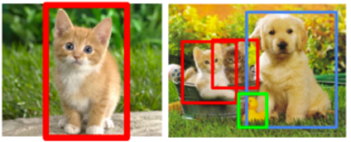
Data Scientists don’t sleep. The competition immediately moved to the next battlefield of object segmentation and classification for embedded image content. The ability to pick out objects inside a crowded image is a precursor to fantastic capabilities, like image captioning, where the model describes a complex image in full sentences. The initial effort to translate full-image recognition to object classification involved different means of localization to efficiently derive bounding boxes around candidate objects. Each bounding box is then processed with a CNN to classify the single object inside the box. A direct pixel-level dense prediction without preprocessing was, for a long time, a highly sought-after prize.
Figure 2. Use bounding box to classify embedded objects in an image

In 2016, a UC Berkeley group, led by E. Shelhamer, achieved this goal using a technique called Fully Convolutional Neural Network. Instead of using convnet to extract visual features followed by fully connected layers to classify the input image, the fully connected layers are converted to additional layers of convnet. Whereas the fully connected layers completely lose all information on the original pixel locations, the cells in the final layer of a convnet are path-connected to the original pixels through a construct called receptive fields.
Figure 3. During the forward pass, a convnet reduces raw pixel information to condensed visual features which can then be effectively classified using fully connected neural network layers. In this sense, the feature vectors contain the semantic information derived from looking at the image as a whole.
 source: https://people.eecs.berkeley.edu/~jonlong/long_shelhamer_fcn.pdf
Figure 4. In dense prediction, we want to both leverage the semantic information contained in the final layers of the convnet and assign the semantic meaning back to the pixels that generated the semantic information. The upsampling step, also known as the backward pass, maps the feature representations back onto the original pixels positions.
![]()
source: https://people.eecs.berkeley.edu/~jonlong/long_shelhamer_fcn.pdf
The upsampling step is something of great interest. In a sense, it deconvolutes the dense representation back to its original resolution and the deconvolution filters can be learned through Stochastic Gradient Descent, just like any forward pass learning process. A good visual demonstration of deconvolution can be found here. The most practical way to implement this deconvolution step is through bilinear interpolation, as discussed later.
The best dense prediction goes beyond just upsampling the last and coarsest convnet layer. By fusing results from shallower layers, the result becomes much more finely detailed. Using a skip architecture as shown in Figure 4, the model is able to make accurate local predictions that respect global structure. The fusion operation is based on concatenating vectors from two layers and perform a 1 x 1 convolution to reduce the vector dimension back down again.
Figure 5. Fuse upsampling results from shallower layers push the prediction limits to a finer scale.

source: https://people.eecs.berkeley.edu/~jonlong/long_shelhamer_fcn.pdf
LABELED DATA
As is often the case when working with Deep Learning, collecting high-quality training data is a real challenge. In the image recognition field, we are blessed with open source data from PASCAL VOC Project. The 2011 dataset provides 11,530 images with 20 classes. Each image is pre-segmented with pixel-level precision by academic researchers. Examples of segmented images can be found here.
OPEN SOURCE MODELS
Computer vision enthusiasts also benefit hugely from open source projects which implement almost every exciting new development in the deep learning field. The author’s group posted a Caffe implementation of FCNN. For keras implementations, you will find no fewer than 9 FCN projects on GitHub. After trying out a few, we focused on the Aurora FCNproject, which started running with very little modifications. The authors provided rather detailed instruction on environment setup and downloading of datasets. We chose the AstrousFCN_Resnet50_16s model out of the six included in the project. The training took 4 weeks on a two Nvidia 1080 card cluster, which was surprising but perhaps understandable given the huge number of layers. The overall model architecture can be visualized by either a JSON tree or with PNG graphics, although both are too long to fit on one page. The figure below shows just one tiny chunk of the overall model architecture.
Figure 6. Top portion of the FCN model. The portion shown is less than one-tenth of the total.

source: https://github.com/aurora95/Keras-FCN/blob/master/Models/AtrousFCN_Resnet50_16s/model.png
It is important to point out that the authors of the paper and code both leveraged established image recognition models, generally the winning entries of the ImageNet competition, such as the VGG nets, ResNet, AlexNet, and the GoogLeNet. Imaging is the one area where transfer learning applies readily. Researchers without the near infinite resources found at Google and Microsoft can still leverage their training results and retrain high-quality models by adding only small new datasets or make minor modifications. In this case, the proven classification architectures named above are modified by stripping away the fully connected layers at the end and replaced with fully convolutional and upsampling layers.
RESNET (RESIDUAL NETWORK)
In particular, the open source code we experimented with is based on Resnet from Microsoft. Resnet has the distinction of being the deepest network ever presented on ImageNet, with 152 layers. In order to make such a deep network converge, the submitting group had to tackle a well-known problem where error rate tends to rise rather than drop after a certain depth. They discovered that by adding skip (aka highway) connections, the overall network converges much better. The explanation lies with the relative ease in training intermediates to minimize residuals rather the originally intended mapping (thus the name Residual Network). The figure below illustrates the use skip connections used in the original ResNet paper, which are found in the open source FCN model derived from ResNet.
Figure 7a. Resnet uses multiple skip connections to improve the overall error rate of a very deep network
![]()
source: https://arxiv.org/abs/1512.03385
Figure 7b. Middle portion of the Aurora model displaying skip connections, which is a characteristic of ResNet.

source: https://github.com/aurora95/Keras-FCN/blob/master/Models/AtrousFCN_Resnet50_16s/model.png
The exact intuition behind Residual Network is less than obvious. There is plenty good discussion in this Quora blog.
BILINEAR UPSAMPLING
As alluded to in Figure 4, at the end stage the resolution of the tensor must be brought back to original dimension using an upsampling step. The original paper stated that a simple bilinear interpolation is fast and effective. And this is the approach taken in the Aurora project, as illustrated below.
Figure 8. Only a single upsampling stage was implemented in the open source code.

source https://github.com/aurora95/Keras-FCN/blob/master/Models/AtrousFCN_Resnet50_16s/model.png
Although the paper authors pointed out the improvement achieved by use of skips and fusions in the upsampling stage, it is not implemented by the Aurora FCN project. The diagram for the end stage illustrates that only a single up sampling layer is used. This may leave room for further improvement in error rate.
The code simply makes a TensorFlow call to implement this upsampling stage:
X = tf.image.resize_bilinear(X, new_shape)
ERROR RATE
The metrics used to measure segmentation accuracy is intersection over union (IOU). The IOU measured over 21 randomly selected test images are:
[ 0.90853866 0.75403876 0.35943439 0.63641792 0.46839113 0.55811771
0.76582419 0.70945356 0.74176198 0.23796475 0.50426148 0.34436233
0.5800221 0.59974548 0.67946723 0.79982366 0.46768033 0.58926592
0.33912701 0.71760929 0.54273803]
These have a mean of 0.585907. This mean is very close to the number published in the original paper. The pixel level classification accuracy is very high at 0.903266, meaning when a pixel is classified as certain object type, it is correct about 90% of the time.
CONCLUSION
The ability to identify image pixels as members of a particular object without a pre-processing step of bounding box detection is a major step forward for deep image recognition. The techniques demonstrated by Shelhamer’s paper achieves this goal by combining coarse-level semantic identification with pixel-level location information. This technique leverages transfer learning based on pre-trained image recognition models that were winning entries in the ImageNet competition. Various open source project replicated the results. Certain implementations require extraordinarily long training time.


